Elo Rating Predictions for KataGo Networks through Logistic Regression
In this post, I explore how a logistic regression model can predict the Elo ratings for two versions of KataGo networks, 18b and 28b. Using the Elo rating system, which assesses performance based on game outcomes, I aim to understand the strengths of these networks. The logistic regression approach offers a way to estimate these ratings, providing insights into each network’s strength in Go.
Network Descriptions
In my exploration, I focus on two distinct KataGo networks, known as 18b and 28b. Both networks are built upon the advanced nested residual bottleneck architecture, which significantly influences their strategic capabilities in Go.
- 18b Network: The 18b network features 18 blocks and is actively developed through collaborative efforts on the KataGo Distributed Training Server. It represents a mature model with extensive training, optimized for both efficiency and strategic depth.
- 28b Network: The 28b network, with its 28 blocks, represents an evolution towards more sophisticated and robust gameplay analysis. While it’s still in the development phase, a preliminary version of the 28b network has been made accessible for testing and feedback through the computer go Discord channel.
This comparative analysis between the 18b and 28b networks seeks to shed light on the advancements in training methodologies and the potential improvements in gameplay strategy as the 28b network progresses.
Elo Rating System
In the context of KataGo networks, Elo ratings emerge from the networks’ performances against each other, reflecting their relative strengths and weaknesses. The calculation of an Elo rating is grounded in the outcomes of games played, adhering to the formula:
\[\text{Elo} = -400 * \log_{10}(-1 + (N / M))\]Here, \(N\) represents the total number of games played, and \(M\) stands for the victories achieved. This mathematical approach transforms the win/loss record into a singular value, making it easier to gauge a network’s prowess at a glance.
Purpose of Modeling Elo Ratings
Modeling Elo ratings for the KataGo networks, particularly the 18b and 28b versions, serves a critical function in evaluating their performance across diverse gameplay conditions. Direct calculations of Elo ratings using traditional methods are resource-intensive, especially when examining a broad spectrum of playouts options.
Logistic Regression Analysis
The foundation of this study is the application of logistic regression to predict the win probabilities in games between the 18b and 28b KataGo networks. This statistical method is well-suited for my goal, as it models the likelihood of binary outcomes—winning or losing—based on input variables.
Within my Elo rating model, the logistic regression equation is expressed as:
\[f(x,y) = {1 \over {1 + \exp({-b-w_1 \ln(x) - w_2 \ln(y)})}}\]In this equation:
- \(f(x,y)\) indicates the probability of the 28b network winning against the 18b network, with \(x\) and \(y\) being their respective maximum visit counts.
- \(b\) is the model’s baseline bias, setting the initial win probability.
- \(w_1\) and \(w_2\) are coefficients that measure the effect of each network’s configuration on the game outcome.
- The logarithmic terms, \(\ln(x)\) and \(\ln(y)\), adjust the impact of maximum visits in a proportional manner.
This logistic regression model allows me to transform the dynamics of Go gameplay into quantifiable probabilities. By tuning this model with data from actual games, I gain insights into the effects of network settings on the balance of competition, providing a detailed view of each network’s performance in various scenarios.
Model Formulation for Elo Rating Estimation
Advancing from the logistic regression analysis, I refine the Elo rating estimation with a model that incorporates the win probabilities from the regression. Integrating the logistic function into the Elo calculation enables a more accurate depiction of competitive strength:
\[\text{Elo} = -400 * \log_{10}(-1 + (1 / f(x,y)))\]Transforming this with the logistic regression result, the Elo rating equation becomes:
\[\text{Elo} = {400(b+w_1 \ln(x) + w_2 \ln(y)) \over {\ln(10)}}\]This approach uses the logistic regression output—\(f(x,y)\)—to compute Elo ratings, reflecting the effects of network configurations on competitive outcomes.
Refining the Model: Active Learning Approach
To enhance the accuracy of my logistic regression model in predicting the Elo ratings for the 18b and 28b KataGo networks, I employ an active learning strategy. This approach systematically refines the model by iteratively incorporating new data points that are expected to provide the most valuable information.
Active Learning Process:
- Initial Sampling: Begin with a random selection of max visit combinations within a predefined range for the initial set of games, establishing a baseline model.
- Candidate Generation: For each iteration, generate a set of 50 new candidate combinations of max visits for the 18b and 28b networks.
- Expected Improvement Calculation: Evaluate each candidate by calculating its Expected Improvement (EI) over the current model predictions. The EI metric captures the potential value of each candidate in enhancing the model’s performance, factoring in the degree of uncertainty in the prediction.
Here, \(T\) represents a temperature parameter that introduces a controlled level of randomness into the selection process, encouraging exploration of less certain outcomes.
- Selection of Top-K Candidates: From the pool of candidates, select the top \(K\) combinations with the highest EI scores. These selections are expected to yield the most significant insights when added to the training data.
- Model Update: Play games using the selected max visit combinations, observe the outcomes, and update the logistic regression model with these new data points. This step incrementally improves the model’s predictive accuracy and reliability.
By continuously cycling through this active learning loop, I systematically enhance the model’s understanding of the relationship between max visit settings and game outcomes. This iterative process ensures that my model remains adaptive and increasingly reflective of the true dynamics between the 18b and 28b networks, leading to more precise and actionable Elo rating estimations.
Optimizing Exploration with Temperature-Controlled Expected Improvement
The concept of temperature in my active learning loop plays a crucial role in balancing exploration with exploitation. By adjusting the temperature parameter, I modulate the degree of randomness in selecting new data points for model refinement, ensuring a dynamic and adaptive learning process.
Temperature Dynamics: The temperature term, \(T\), is strategically decreased over time, following a linear decay. This approach is designed to encourage a higher degree of exploration in the early stages of model training, where the broader search for informative data points is beneficial. As the model becomes more refined, the focus shifts towards exploitation, honing in on areas of the parameter space that are most likely to enhance model accuracy around \(\text{Elo} = 0\).
The temperature is adjusted according to the formula:
\[T = k \cdot {(N_\text{iter} - i) \over N_\text{iter}} \cdot \text{rand}[0,1]\]In this formula:
- \(k\) is a scaling factor that determines the overall level of randomness introduced by the temperature.
- \(N_{\text{iter}}\) represents the total number of iterations planned for the active learning loop, setting the timeframe over which the temperature will decay.
- \(i\) denotes the current iteration, allowing the temperature to decrease linearly as the model progresses through successive rounds of refinement.
- \(\text{rand}[0,1]\) introduces a random element to the temperature adjustment.
This temperature-controlled mechanism ensures that my learning process remains agile, continuously adapting to the evolving landscape of the model’s performance. By fine-tuning the balance between exploring new possibilities and exploiting known information, I can achieve a more robust and accurate Elo rating prediction model for the KataGo networks.
Experiment
The experiment was set up using KataGo v1.14.0 with an OpenCL backend, executed on a MacBook M3 Pro Max. The objective was to assess the Elo rating predictions of the 18b and 28b networks through a series of controlled simulations.
Detailed Experimental Parameters:
- Top-K Selection: I employed a selection strategy focusing on the top 8 points (\(K=8\)) for analysis, ensuring a targeted approach to data gathering.
- Temperature Adjustment: The experiment incorporated a temperature control parameter (\(k=2\)), crucial for managing the exploration-exploitation balance during the learning process.
- Iterative Process: The methodology involved 120 iterations (\(N_\text{iter}=120\)), each contributing to the incremental refinement of the model.
For an in-depth understanding, refer to the detailed source code.
KataGo Network Configurations:
- A uniform setting of
numSearchThreads = 1was maintained to ensure consistency in performance evaluation across networks. - The 18b network:
kata1-b18c384nbt-s9131461376-d4087399203.bin.gz. - The 28b network:
b28c512nbt-s4302634752-d4157365465.bin.gz.
Detailed Analysis of Experimental Results
The experimental phase yielded an extensive dataset, capturing the evolving relationship between the logistic regression model’s coefficients and bias over a series of 120 iterations. This data provides a window into the model’s learning process, reflecting how it adjusts its parameters in response to new information.
Visualization of Model Dynamics:
An illustrative graph showcases the variation in the model’s coefficients and bias throughout the experiment.
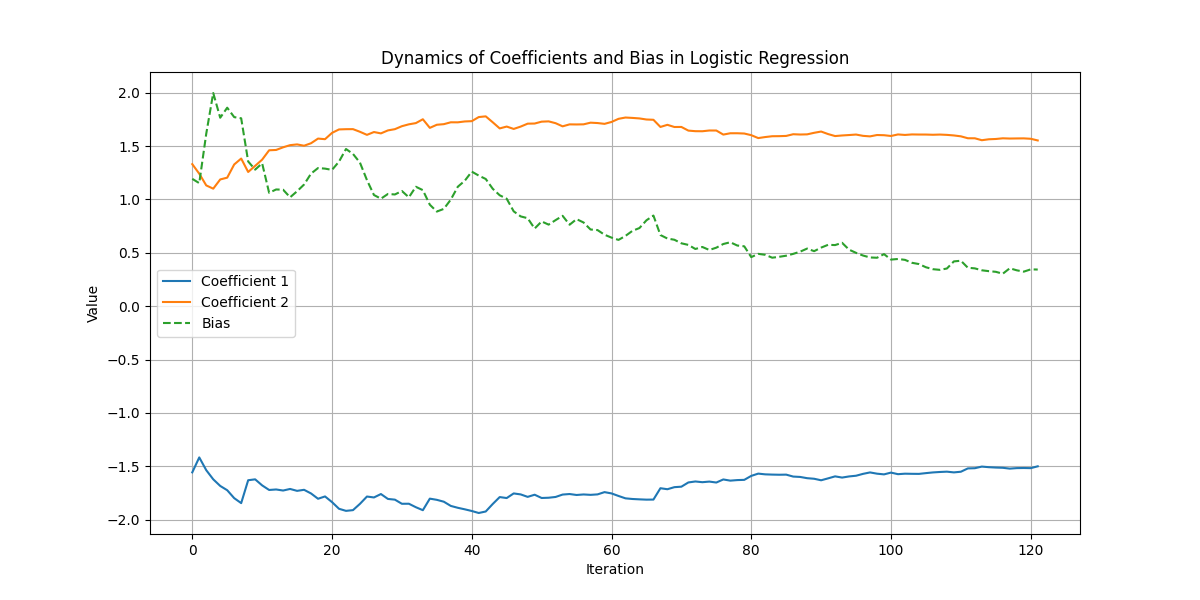
On this graph:
- The x-axis tracks the progression of iterations, marking the temporal aspect of the learning process.
- The y-axis quantifies the values of the coefficients and bias at each iteration.
- The plotted lines represent the evolution of two coefficients and the bias, visually narrating the model’s calibration journey.
Quantitative Insights:
The final bias and coefficients are listed below:
- Coefficients: \((w_1, w_2) = (-1.49987981, 1.55287902)\).
- Bias: \(b = 0.34352172\).
Interpretative Scatter and Contour Plots:
Another set of visuals provides a scatter plot alongside a contour plot, enriching my interpretation of the Elo rating model’s predictions.
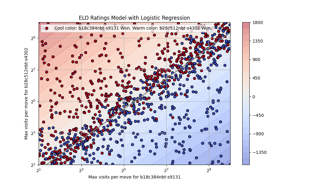
The scatter plot:
- Features points representing the outcomes of simulated games between the 18b and 28b networks under varied visit conditions.
- Utilizes a color-coding scheme to differentiate victories, with cool colors indicating wins for the 18b network and warm colors for the 28b network, providing an intuitive understanding of each network’s performance across different scenarios.
The contour plot:
- Introduces a gradient background that acts as a decision boundary, effectively mapping the zones where the model forecasts a competitive edge for one network over the other.
- Highlights the regions of increased prediction confidence away from the boundary, where the color intensity signifies a stronger likelihood of victory for the predicted winner.
Together, these visual analyses not only validate the logistic regression model’s predictive accuracy but also offer strategic insights into the relative strengths of the 18b and 28b networks, guiding future enhancements and optimization approaches.
Comprehensive Benchmark Analysis
The KataGo benchmarking utility, a specialized subcommand, is instrumental in evaluating the networks’ efficiency by measuring the number of positions processed per second under predefined conditions.
Benchmark Results: For a consistent comparison, I set the search thread count to one for both networks. The results highlight the computational performance of each network in handling game positions:
| Network | Threads | Visits/s |
|---|---|---|
| 18b | 1 | 99.76 |
| 28b | 1 | 64.85 |
These figures underscore the differences in processing efficiency between the 18b and 28b networks, offering insights into their operational capabilities.
Equilibrium Points in Elo Ratings
My analysis identifies specific conditions under which the 18b and 28b networks exhibit equivalent performance levels, reflected in a zero Elo rating difference. This equilibrium is crucial for understanding the balance point in network capabilities.
Equilibrium Conditions:
The table below details the max visits and corresponding times at which the networks achieve parity in performance:
| 18b Visits | 18b Time (s) | 28b Visits | 28b Time (s) |
|---|---|---|---|
| 4.00 | 0.0401 | 3.06 | 0.0472 |
| 8.00 | 0.0802 | 5.97 | 0.0921 |
| 16.00 | 0.1604 | 11.67 | 0.1800 |
| 32.00 | 0.3208 | 22.79 | 0.3514 |
| 64.00 | 0.6415 | 44.51 | 0.6864 |
| 128.00 | 1.2831 | 86.94 | 1.3406 |
| 256.00 | 2.5662 | 169.81 | 2.6185 |
| 512.00 | 5.1323 | 331.69 | 5.1147 |
These conditions provide a framework for predicting scenarios where the networks are expected to perform with equal strength, offering a nuanced understanding of their capabilities.
Optimizing Search Threads and Understanding Elo Costs
While both the 18b and 28b networks show comparable performance with a single search thread in terms of time efficiency, it’s crucial to recognize that the 18b network might outperform the 28b when optimized thread counts are used. The table below presents the ideal number of search threads for each network, highlighting their respective visits per second.
| Network | Thread | Visits/s |
|---|---|---|
| 18b | 16 | 378.63 |
| 28b | 12 | 164.94 |
With the optimized thread count, the 28b network achieves 2.54 times the visits, while the 18b network sees an increase to 3.80 times its single-thread performance.
However, this optimization is based on historical data, where the Elo cost formula, as described in KataGo’s documentation, is calculated by:
numThreads * 7.0 * pow(1600.0 / (800.0 + baseVisits), 0.85);
This calculation might not accurately reflect the current efficiency of the KataGo engine, especially with the advancements in the 18b and 28b networks. Several critical questions remain open for exploration:
- Elo Cost and Thread Count: Investigating how the relationship between Elo ratings and search thread counts evolves with newer versions of the KataGo engine is crucial.
- Search Thread Optimization: There is potential to improve the efficiency of multithreaded searches for both the 18b and 28b networks, which could lead to significant performance gains.
- Parameter Tuning: Identifying the most effective KataGo parameters for these networks could further enhance their strategic gameplay capabilities.
Conclusion
My study on modeling Elo ratings for KataGo’s 18b and 28b networks through logistic regression has provided valuable insights into their strategic performance. The analysis highlights the potential for optimizing search threads and adjusting parameters to enhance KataGo capabilities.